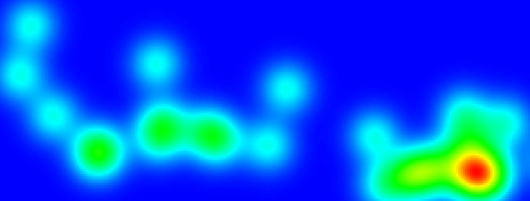
Kernel Density Maps are a way to look at the relative density of point data as spread over an area. The Cartographica Kernel Density Map option uses a highly-accurate Kernel for its analysis. By default, the kernel density analysis uses a set of "reasonable" parameters, however an advanced version of the feature is available by holding down the Option key on your keyboard while selecting the menu item that allows you to change those defaults.
You can make a Kernel Density map on any point layer. This creates an analysis layer (basically a bitmap, at least visually, but it's actually a "cell" system where each "cell" contains the value for the area bounded by the rectangle the cell contains).
Depending on your particular data, you may find it helpful to either move this layer to the bottom of your layer stack, or use the Styles item to change the layer opacity to be more transparent.
To create a Kernel Density Map using the default parameters:
From the layer stack, select a single point layer in your mapset for which to analyze the density.
Select the Zoom level for the Kernel Density Map in the Map window by zooming in to the view you want. The default Kernel Density analysis is performed on the area in the Map View at time that you select the command.
Choose >
After the analysis is complete, the graphical map will be added as a layer to the mapset.
To create a Kernel Density Map specifying the precise parameters:
From the layer stack, select a single point layer in your mapset from which to analyze the density.
Select the Zoom level for the Kernel Density Map in the Map window by zooming in to the view you want.
Hold the Option key and choose >
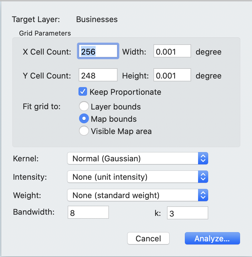
The Kernel Density Map Options window appears.
Select the options for this analysis:
Target Layer is the point layer to be analyzed.
X Cell Count,Y Cell Count,Width, and Height provide a way to change the number (and thus size, or vice versa) of the cells used in the calculation. The width and height parameters conform to whatever the target layer's projection is, so if the projection is in State Plane (feet), feet will be the size. Cartographica analyzes the field using a grid of cells spread evenly across the field. By setting the count of the grid cells, you can determine the coarseness of the grid that is used.
To change this, either choose the width and height in number of cells, or in map units (here in the example, it's in degrees, but if your map layer's CRS is set to feet or meters, the parameter will be in those units).
If the Keep Proportionate check box is checked, Cartographica will adjust the width to match the height you enter, and vice-versa. For a disproportionate grid, then uncheck the box.
Fit grid to allows for adjustment of the coverage area of the grid to one of the following:
Layer Bounds constrains to the data in the layer.
Map Bounds constrains to the entire map.
Visible Map Area constrains to the area currently shown on the map view (where this is useful if you want the KDM to go beyond the boundary of the current map to provide some context by means of a smooth drop-off.
Kernel allows for the specification of the kernel used for the analysis
Table 8.1. Available Kernels
Normal (Gaussian) Unbounded. Each data point contributes something to every cell Quartic (or Spherical) Bounded. Approximates the normal with a constant k. Exponential (Negative) Much more weight is given to the center points Triangular (Conic) Linear decay with distance Uniform (Flat) Bounded. Value is k or 0 Paraboloid/quadratic (Epanechnikov) Bounded, more spread out than Quartic (or Spherical) and used in ArcGIS Intensity and Weight allow you to assign columns in the layer from which these values are retrieved. Without changing these parameters, the defaults are to use an intensity and weight of 1.0, which gives each point equal weight. These two values are multiplied and then added into the cell for the map. Thus, a cell that contains a single point with a weight of 2 and an intensity of .5 has a value of 1.
For example, if you have data that is a list of duck-blind positions with the number of ducks seen in a one hour period, you would set the intensity to the count and that would give you an idea where the ducks are concentrated.
Bandwidth is the radius of the band that the point affects in cells and determines the decay of the value from the central point. If the bandwidth is set to 8, then little or no effect will be generated by the 8th cell from the point. If you set this number larger, the effect will spread out to a wider radius.
k is a parameter specific to a particular kernel function. See Table 8.1, “Available Kernels” for details.
Once you have made your selections click and the Kernel Density Map is created and added to the map as a new analysis layer.