When working with Digital Elevation Model (or DEM) data, there is frequently the need to perform some analysis of the elevation data and how it relates to its surroundings. The > command is intended to provide much of that capability in Cartographica. Based upon the GDAL libraries, Cartographica can perform a number of processing steps, including:
Hillshade (shaded relief)
Slope
Aspect
Color Relief
Terrain Ruggedness Index (TRI)
Terrain Position Index (TPI)
Roughness
Cartographica performs these functions based on the selected layer or layers. As such, multiple raster layers can either be merged together and then analyzed, or they may be analyzed by selecting multiple layers and then choosing > .
Processing Height Raster Layers
Select the layer or layers to be processed in the Layer Stack
Choose >
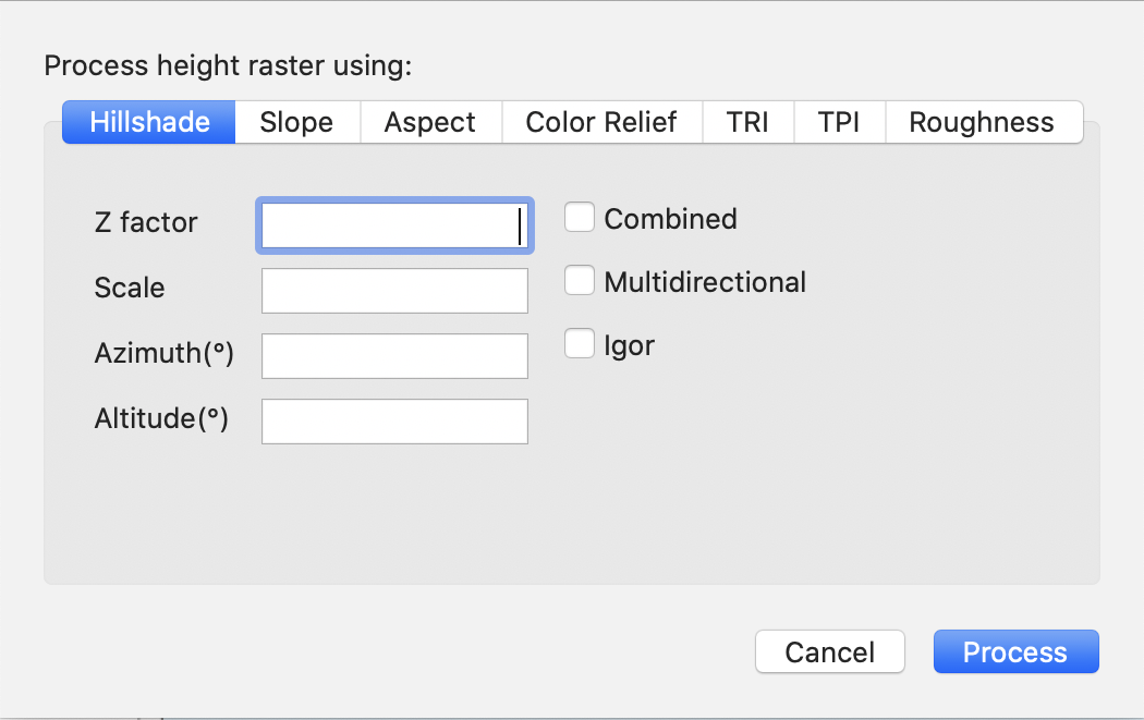
The Process Height Raster sheet will come up
Choose the type of processing you would like by selecting one of the tabs in the sheet
If there are options in the window, you may fill those in and then click to perform the processing
A new layer will be created in the Layer Stack with the output of the processing
All of the algorithms for these calculations come from recent versions fo the GDAL libraries. Here we present a summary of the functionality and parameters, based on the documentation.
The Hillshade processor creates an 8-bit raster with a shaded relief effect. It is mostly useful for visualizing terrain. Adjustments can be made to the azimuth and altitude of the light source, and scaling information can be added to account for differences between the vertical and horizontal units.
![[Warning]](Graphics/warning.svg) | |
Many of these algorithms expect that the X, Y and Z scales are the same in the original data. For data that is consistently in meters (x and y in a local projected coordinate system in meters, and the DEM data itself in meters), there's no need to adjust the scaling. However, in the case the the source layer is in Lat/Long (for example), the scale will need to be set to 111120 if the DEM data are in meters and 370400 if they are in feet. |
Table 9.1. Hillshade Parameters
| Z factor | Vertical exaggeration used to pre-multiply the elevation data. This may be necessary when trying to accentuate the height differences, for example for areas that are relatively flat. |
| Scale | Ratio of the vertical units to horizontal. (See note above) |
| Azimuth(°) | Azimuth of the light source, in degrees. 0 is from the top the raster image, 90 from the right side (East often). The default value is 315° is commonly used for shaded maps, and should be considered a standard. |
| Altitude(°) | Altitude of the light source, in degrees. 90 if the light comes directly above the DEM, 0° if it is raking light. The default value of 45° is commonly used for shaded maps. |
| Combined | Use a combination of oblique and slope shading. If not checked, it will use just oblique shading. |
| Multidirectional | Use Multidirectional shading, a combination of hillshading illuminated from 225°, 270°, 315° and 360°. Applies the formula from Multidirectional, oblique-weighted, shaded-relief image of the Island of Hawaii from the USGS. |
| Igor | Shading which attempts to minimize effects on other map features by rendering a "softer" hillshade. Uses the techniques covered in Igor's hillshading method from Maperitive. |
Creates a 32-bit float raster with slope values as either percent or degrees. Where appropriate a no-data value of -9999 is used.
Table 9.2. Slope Parameters
| Scale | Ratio of the vertical units to horizontal. (See note above) |
| Slope as Percent | Checked if the output values should be as a percent, otherwise they are in degrees |
Creates a 32-bit float raster with values between 0° and 360° representing the azimuth that slopes are facing. The definition of the azimuth is such that:
Table 9.3. Aspect Parameters
Angle | Azimuth | Trigonometric |
|---|---|---|
| 0° | Facing North | Facing East |
| 90° | Facing East | Facing North |
| 180° | Facing South | Facing West |
| 270° | Facing West | Facing South |
This presumes that the raster input is North at the top when the data is processed). Where appropriate a no-data value of -9999 is used.
Table 9.4. Aspect Settings
| Trigonometric | Provide trigonometric angle instead of azimuth (see table above) |
| Zero for Flat | Return 0 for areas with a flat slope, instead of -9999 |
![[Note]](Graphics/note.svg) | |
By checking both of these options (Trigonometric and Zero for Flat), the
aspect returned should be identical to the one from GRASS
|
This process creates a 3-band (RGB) or 4-band (RGBA) raster with values that are computed from the elevation and from the color configuration, which provides a mapping from various elevation values to a corresponding desired color. Color blending is handled based on the settings in the Color Blending Mode table, and an optional Alpha channel can be added, which affects both blending and the use of exact color (in the case of exact color, non-matching colors are transparent).
Table 9.5. Color Blanding Modes
| Blending Mode | Effect |
|---|---|
| Exact Match | Only exactly matching colors are set. All other values result in (0,0,0) or (0,0,0,0) if alpha is enabled |
| Nearest Color | The color in the Height/Color map which is nearest is used |
| Smooth Blend | A proportionate blend between the nearest 2 colors is used |
Height/Color mapping can be provided either by manually entering items into the table or by loading color mapping files. The color mapping files are simple text files which have a list of heights and their corresponding color values. The values column (leftmost) contains the elevation value, which may be a floating point value, a percentage value (appended with %), or nv to indicate no data (no value). The color columns may contain a textual color value (currently supported values are: white, black, red, green, blue, yellow, magenta, cyan, aqua, grey/gray, orange, brown, purple/violet and indigo), an RGB triple (red, green, blue), or an RGBA quad (red, green, blue, alpha). In the case of the multi-values, the values range from 0 to 255 and may be separated by spaces, commas, tabs, or colons (:). Finally, the absence of an alpha value denotes full opacity (255).
3500 white
2500 235:220:175
50%  190 185 135
700  240 250 150
0    50  180  50
nv   0   0    0   0
To specify Height/Color mapping manually
Click to add a new row
Click in the Height Level of the new row and put in an elevation or %age
Click in the corresponding Color Specifier and put in a color name, or 3 or 4 values from 0-255 (3 for RGB, 4 for RGBA)
Value sets may be saved to a file by choosing > from the drop-down menu beneath the table
Value sets may be loaded from a file by choosing > from the drop-down menu beneath the table
This process creates a single-band raster with values computed based on the elevation and the mean difference between a central pixel and its surrounding cells. For details, see Multiscale Terrain Analysis of Multibeam Bathymetry Data for Habitat Mapping on the Continental Slope.
This process creates a single-band raster with values computed based on the elevation and difference between a central pixel and the mean of its surrounding cells (also from Multiscale Terrain Analysis of Multibeam Bathymetry Data for Habitat Mapping on the Continental Slope).
This process creates a single-band raster with values computed based on the elevation and the largest inter-cell difference of a central pixel and its surrounding cells (also from Multiscale Terrain Analysis of Multibeam Bathymetry Data for Habitat Mapping on the Continental Slope).